What is Fern?
Fern optimizes pipelines built from sequences of function calls. In particular, Fern fuses function calls, and produces code that evaluates operations back-to-back on small chunks of data as opposed to entire outputs. Fern accomplishes this by requiring functions to declare how they produce and consume data.
Fern's core idea is that that fused code naturally separates concerns: inner loops handle computation and hardware-specific logic, while outer loops manage data movement. Fern uses black-box subroutines to perform computations and uses simple dataflow analysis to generate outer loops.
Our paper on Lightweight and Locality-Aware Composition of Black-Box Subroutines discusses Fern's design philosophy in detail.
Getting Started
To get started with Fern, take a look at the installation instructions.
The tutorial walks through several example Fern programs to help you understand how it works in practice.
Talk
You can also watch our CppCon talk about Fern. Fern has evolved quite a bit since then, but the design philosophy at its core has remained the same.
An Introduction to Operator Fusion
A Simple Example
Consider a simple function that takes in an array of floats a,
and adds 1 to each element, storing its output in b:
void add_1(float * a, float *b, int N){
    for (int i = 0; i < N; i++){
        b[i] = a[i] + 1;
    }
}
To perform 2 to elements to an array, we can simply call add_1 twice:
    float * a  = (float *) malloc(N * sizeof(float))
    float * b  = (float *) malloc(N * sizeof(float))
    float * c  = (float *) malloc(N * sizeof(float))
    add_1(b, a, N);
    add_1(c, b, N);
or, we can implement a special add_2 function:
void add_2(float * a, float *b, int N){
    for (int i = 0; i < N; i++){
        b[i] = a[i] + 2;
    }
}
and simply call it:
    float * a  = (float *) malloc(N * sizeof(float))
    float * c  = (float *) malloc(N * sizeof(float))
    add_2(c, a, N);
The add_2 function not only uses less memory, requiring no allocation for an
intermediate, it also takes advantage of locality. Each float is loaded once
and all operations are applied immediately, when the data is ready. This
technique of applying a sequence of operations back-to-back on susbets of data
rather than computing entire intermediate outputs is called operator fusion.
Traditionally, your favorite compiler runs a fusion pass, bringing computations into the same outer-loop scope when it can determine that the transformation is correct. While these passes typically fuse at single data element granularity, one can also generalize this idea to instead think about fusion happening at different granularities (4 elements, 8 elements, tiles of data, etc.).
Operator Fusion in Practice
High-performance applications are often built as compositions of function calls, many sourced from mature, highly optimized libraries like CBLAS. On Apple’s M3 chip, the fastest implementations of the CBLAS interface can be found in frameworks such as Accelerate and Arm Performance Libraries.
CBLAS itself contains several fused interfaces. For example, cblas_sgemm performs a matrix-matrix multiplication with optional transposition and scaling, all in a single call.
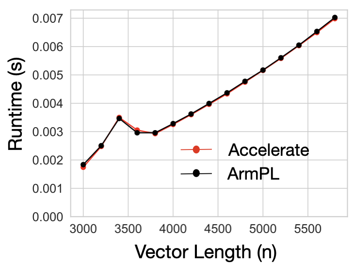
Say we want to compute a General Vector Rank Update (GER) operation expressed as \( A = \alpha (x \times y^T) + A \) where \( A \) is a matrix, \( x \) and \( y \) are vectors, \( \alpha \) is a scalar, and all datatypes are floats. Both Accelerate and ArmPL offer implementations of this operation, and their performance is pretty close.
If we were to comupute a slight variant of our computation, an SGERB \( A = \alpha (x
\times y^T) + \beta A \), we have two options. First,
we can use ArmPL’s fused BLAS extension interfaces that include an sgerb_ subroutine. Or, as
Accelerate has no fused subroutine, we can compose Accelerate’s cblas_sger and cblas_saxpy
subroutines.
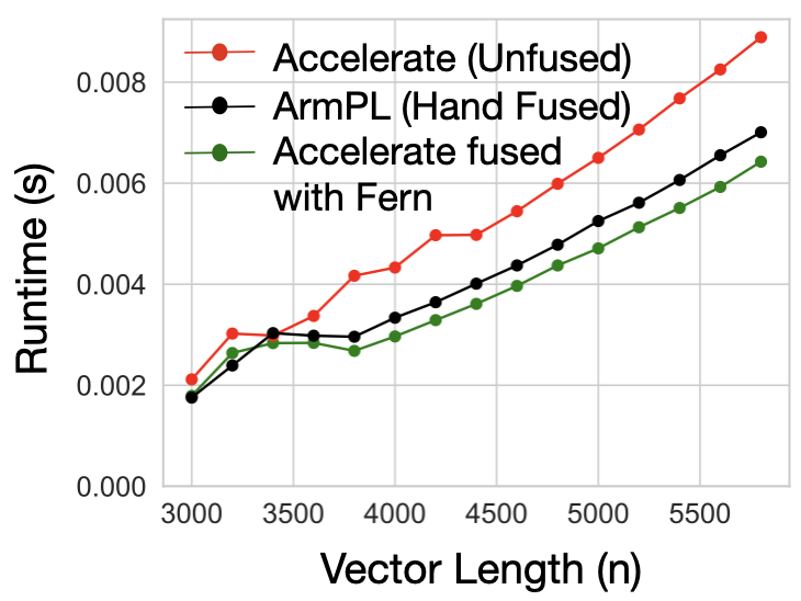
However, the fused ArmPL subroutine is 1.24× (geomean) faster than the composed Accelerate implementation. Since Accelerate already matched ArmPL’s performance on GER, the performance difference between the two implementations on GERB is not due to an under-optimized inner loop or poor instruction selection, but is rather introduced at the point of composition. ArmPL is able to fuse its computation, resulting in the difference that we see.
In our trivial example with add_1, we could quickly write a fused
implementation. However, in this case, we are stuck: each routine cblas_sger
and cblas_saxpy likely contains hundereds of lines of hairy,
architecture-specific code that would be time consuming to rewrite and error prone
to modify. Worse, both ArmPL and Accelerate are propriety frameworks. In fact, the
Accelerate library is the only way to target undocumented, Apple-specific
hardware. If our user wants to use this special hardware, they are tied to the
Accelerate library, which does not have extended BLAS kernels like
sgerb_. But, if our user wants to use fused implementations provided in
the BLAS extension interface, they must use ArmPL.
Instead of using naive subroutine calls for Accelerate, the user can use code generated by Fern, which continues to call Accelerate subroutines, but does so for small tiles of the output at a time. To see how to do this, head to the tutorial.
Installation
Fern is now supported by the Gern repository. Gern adds support for GPUs and contains Fern-style CPU support. Gern is under 🚧 active development 🚧.
Fern is an open-source project available at https://github.com/manya-bansal/gern.
It is written in C++20 and requires CMake version 3.30 or higher to build.
Getting the Repository
First, clone the repository from github.
$ git clone [email protected]:manya-bansal/gern.git
Installing Dependencies
VCPKG
Fern uses vcpkg to manage its
dependencies. Follow the official guide to download and install vcpkg: Get Started with
vcpkg
Once installed, set the VCPKG_ROOT environment variable to point to your
vcpkg directory.
CMake
Fern uses cmake as its build system. Before building Fern, ensure that cmake
is installed on your system. Fern requires cmake 3.30 and above.
You can download the latest version of CMake from the official website: CMake Downloads
Building Fern
Now that VCPKG_ROOT is set and you have downloaded the repository, build the
repository from the gern directory:
$ cmake -DGern_CUDA_ARCH=<89,90..,etc> --preset dev
$ cmake --build build/dev
If -DGern_CUDA_ARCH is not set, none of the GPU kernels will be run during
tests.
Running Tests
To run tests, execute:
$ ctest --test-dir build/dev
Overview
Fern is now supported by the Gern repository. Gern adds support for GPUs and contains Fern-style CPU support. Gern is under 🚧 active development 🚧.
The tutorial walks you through different programs in Fern with increasing complexity. The interface to Fern has changed from the paper, though it is equally powerful.
As opposed to thinking about an explicit separation between algorithm and schedule—where the schedule is a meta-program describing how lowering might proceed—the new interface is a "sketch" of the loop nest the user wants the generated program to have. This sketch is then deterministically lowered into imperative code, with the compiler filling in any details that can be automatically inferred.
The tutorial is organized as follows:
- Making our first function call
- Running our first function call
- Writing a Multi-Function Pipeline
- Understaning Data Structures
- Tiling Programs
- Understanding Legal Tilings
- Tiling Through Reductions
Making a Function Call in Fern
The easiest program to write in Fern is one that makes a single function call:
#include "helpers.h"

int main() {

    // Our first, simple program.
    auto a = mk_array("a");
    auto b = mk_array("b");

    // Gern object that represents a function.
    gern::annot::add_1 add_1;

    Composable program = {
    // the () operator calls the function, and
    // generates a "call site".
        add_1(a, b),
    };

    // The program can now be compiled.
    compile_program(program);
}
Let's look at the different pieces of the add_1 object carefully:
class add_1 : public gern::AbstractFunction {
public:
    add_1()
        : input(new const ArrayCPU("input")),
          output(new const ArrayCPU("output")) {
    }

    /* getAnnotation() returns the data production
     * and consumption pattern of the function.
     * See Tiling Programs in the tutorial for more
     * details if you'd like to skip ahead!
    */
    Annotation getAnnotation() override {
        Variable x("x");

        return annotate(
            Tileable(x = Expr(0), output["size"], step,
                     Produces::Subset(output, {x, step}),
                     Consumes::Subset(input, {x, step})));
    }

     /* getFunction() returns the "C++" signature of the
      * Function that we ultimately use to generate code.
     */
    virtual FunctionSignature getFunction() override {
        FunctionSignature f;
        f.name = "library::impl::add_1"; // <-- Name of the Function
        f.args = {Parameter(input), Parameter(output)}; // <-- Parameters of the function
        // Also contains template arguments which has been left empty.
        return f;
    }

    /**  The file that the function declration lives in, this is included
     *   in the generated file.
     */
    std::vector<std::string> getHeader() override {
        return {
            "cpu-array.h",
        };
    }

protected:
    AbstractDataTypePtr input;
    AbstractDataTypePtr output;
    Variable end{"end"};
    Variable step{"step"};
};
Given our Fern program and the function definition, when we compile the program, we simply get a function that makes a single call (we have not tiled our program yet!):
#include "cassert"
#include "cpu-array.h" // Our include file!

// An automatically generated wrapper function name.
void function_3(library::impl::ArrayCPU& a, library::impl::ArrayCPU& b){
      library::impl::add_1(a, b); // the actual function call!
}
Fern writes the generated code into a file which can then be included in a project, and run like normal.
Running our trivial program
Part one demonstrated how to write a trivial, single function program. To run it, we had to figure out where the generated file lives, include it, compile and then execute it. While this works, it's still annoying to keep including a file into the project just to execute it. To avoid this, Fern also provides an interface for jitting and loading the function pointer, so the code can be compiled and executed more ergonomically.
In this case, we can consider the program as being split into two parts: program definition and program execution.
#include "helpers.h"
#include "library/array/impl/cpu-array.h"

int main() {

    // ***** PROGRAM DEFINITION *****
    // Our first, simple program.
    auto a_def = mk_array("input");
    auto b_def = mk_array("output");

    gern::annot::add_1 add_1;

    Composable program = {
        add_1(a_def, b_def),
    };

    // ***** PROGRAM EVALUATION *****
    // Compile turns a runner object which can be
    // used to run the program.
    auto runner = compile_program(program);

    library::impl::ArrayCPU a(10);
    a.ascending();
    library::impl::ArrayCPU b(10);

    // Evaluate the program. The
    // function takes in a map, and
    // corresponding names of the inputs and
    // outputs. Fern will wire these up correctly!
    runner.evaluate({
        {"output", &b},
        {"input", &a},
    });

    // Make sure we got the right answer.
    for (int i = 0; i < 10; i++) {
        std::cout << "a[" << i << "] = " << a.data[i]
                  << ", b[" << i << "] = " << b.data[i] << std::endl;
        assert(a.data[i] + 1 == b.data[i]);
    }
}
It is worthwhile breaking down what the compile_program helper
is hiding:
inline Runner compile_program(Composable program,
                              std::string name = "program.cpp") {
    Runner runner(program);
    Runner::Options options{
        // Name of the generated file
        .filename = name,
        // Path where the file should be put.
        .prefix = "/home/manya/gern/prez/gern_gen",
        // Paths to include
        .include = " -I /home/manya/gern/prez/library/array/impl"
                   " -I /home/manya/gern/prez/library/matrix/impl",
    };
    // Compile the program!
    runner.compile(options);
    return runner;
}
Runner::Options contains more choices for flags that can be set.
Calling multiple functions
Now that we know how to write and execute Fern pipelines with one function, let's turn our attention to longer pipelines. Here's our previous pipeline, but now with one additional function call:
#include "helpers.h"
#include "library/array/impl/cpu-array.h"

int main() {

    // ***** PROGRAM DEFINITION *****
    // Our first, simple program.
    auto input = mk_array("input");
    auto temp = mk_array("temp");
    auto output = mk_array("output");

    gern::annot::add_1 add_1;

    Composable program({
        add_1(input, temp),
        add_1(temp, output), // <--  New Call
    });

    // ***** PROGRAM EVALUATION *****
    library::impl::ArrayCPU a(10);
    a.ascending();
    library::impl::ArrayCPU b(10);

    auto runner = compile_program(program);
    runner.evaluate(
        {
            {"output", &b},
            {"input", &a},
        });

    // SANITY CHECK
    for (int i = 0; i < 10; i++) {
        assert(a.data[i] + 2 == b.data[i]);
    }
}
As we begin to start writing longer pipelines, there are some rules about writing pipelines must observe:
- All data-structures can be assigned to only once.
This means that we could not used
tempagain as the output of our second call. - All intermediates must be used an input at least once.
Fern would have thrown an error in the case that
tempwas computed, but never used as input.
There are more rules coming up as we write tiled pipelines!
While our program defintion contains temp, you might have noticed that the program
evaluation does not! Indeed, if we look at the generated code, Fern is allocating it:
void function_5(library::impl::ArrayCPU &input, library::impl::ArrayCPU &output) {
    library::impl::ArrayCPU temp = library::impl::ArrayCPU::allocate(0, output.size);

    library::impl::add_1(input, temp);

    library::impl::add_1(temp, output);

    temp.destroy();
}
Fern owns all the temporary/intermediate tensors in a pipeline (and will optimize for reuse of temporaries and hoisting them out). Therefore, only "true" inputs and the "true" output is passed in.
At this point, you might have a lingering question: how did Fern figure out what allocate call to make in the first place?
Demystifying Data Structures
The last piece to unpack before we begin fusing programs is the set of data
structures we've been using in our program definitions. Just like the add_1
function, these data structures are also part of the overall program definition
and contain essential information that Fern uses during code generation and
execution.
Let's look at the array object that mk_array produces:
auto input = mk_array("input");
class ArrayCPU : public gern::AbstractDataType {
public:
    // Array must have a name!
    ArrayCPU(const std::string &name)
        : name(name) {
    }
    // Get the name to use in codegen.
    std::string getName() const override {
        return name;
    }

    // Get the type to use in codegen.
    std::string getType() const override {
        return "library::impl::ArrayCPU";
    }

    // The fields of the array are what we will eventually
    // use to tile our program! In this represenatation
    // x denotes about the start of a subarray, while len
    // denotes the length of the subarray. Gern attaches
    // no semantic meaning to these fields, it just promises
    // to wire then up correctly! The ordering here does play a role!
    std::vector<Variable> getFields() const override {
        return {x, len};
    }
    // How can gern allocate an array?
    FunctionSignature getAllocateFunction() const override {
        return FunctionSignature{
            .name = "library::impl::ArrayCPU::allocate",
            .args = {x, len},
        };
    }
    // How can gern free an array?
    FunctionSignature getFreeFunction() const override {
        return FunctionSignature{
            .name = "destroy",
            .args = {},
        };
    }
    // If gern has a subarray, how can it insert into a parent array?
    FunctionSignature getInsertFunction() const override {
        return FunctionSignature{
            .name = "insert",
            .args = {x, len},
        };
    }

    // If gern wants to extract a subarray, how can it query it?
    FunctionSignature getQueryFunction() const override {
        return FunctionSignature{
            .name = "query",
            .args = {x, len},
        };
    }

protected:
    std::string name;
    Variable x{"x"};
    Variable len{"len"};
};
Similar to our array example, we could have instead used a matrix data structure. Let's take a look at the fieds of the matrix:
  std::vector<Variable> getFields() const override {
        return {x, y, l_x, l_y};
  }
Here, x and y point at the start of a submatrix, while
l_x and l_y denote its height and width. Similar to the
array, we can write a program that uses the matrix!
#include "helpers.h"
#include "library/matrix/annot/cpu-matrix.h"
#include "library/matrix/impl/cpu-matrix.h"

    int
    main()
{
    // ***** PROGRAM DEFINITION *****
    auto input = mk_matrix("input");
    auto output = mk_matrix("output");
    auto temp = mk_matrix("temp");

    annot::MatrixAddCPU add_1;

    Composable program({
        add_1(input, temp),
        add_1(temp, output),
    });

    // ***** PROGRAM EVALUATION *****
    library::impl::MatrixCPU a(10, 10, 10);
    a.ascending();
    library::impl::MatrixCPU b(10, 10, 10);

    auto runner = compile_program(program);
    runner.evaluate({
        {"input", &a},
        {"output", &b},
    });

    // ***** SANITY CHECK *****
    for (int i = 0; i < a.col; i++)
    {
        for (int j = 0; j < a.row; j++)
        {
            assert(a(i, j) + 2 == b(i, j));
        }
    }
}
Tiling a Multi-Function Program
Finally, we can start rewriting tiling programs and producing fused variants.
Let's go back to the annotation function that we saw previously.
   Annotation getAnnotation() override {
        Variable x("x");
        return annotate(
            // Tilable tells us what dimensions of the output
            // can be tiled.
            Tileable(x = Expr(0), output["size"], step,
                     // Produces indicates what subset (pointed at
                     // by the fields we saw in the last chapter)
                     // of the output we are describing.
                     Produces::Subset(output, {x, step}),
                     // What subsets of the input do we need to
                     // consume to produce the required output subset?
                     Consumes::Subset(input, {x, step})));
    }
Now to generate a fused version, we simply tile the output's dimension! As expected, only fields marked as tileable can be tiled.
#include "helpers.h"
#include "library/array/impl/cpu-array.h"

using namespace gern;

int main() {

    // ***** PROGRAM DEFINITION *****
    // Our first, simple program.
    auto input = mk_array("input");
    auto temp = mk_array("temp");
    auto output = mk_array("output");
    Variable t("t");

    gern::annot::add_1 add_1;

    Composable program({
        // Tile the output!
        // t indicates what the tile
        // size should be
        Tile(output["size"], t)(
            add_1(input, temp),
            add_1(temp, output)),
    });

    // ***** PROGRAM EVALUATION *****
    library::impl::ArrayCPU a(10);
    a.ascending();
    library::impl::ArrayCPU b(10);
    int64_t t_val = 2;

    auto runner = compile_program(program);
    runner.evaluate(
        {
            {"output", &b},
            {"input", &a},
            {"t", &t_val}, // <-- t must also be provided now!
        });

    // SANITY CHECK
    for (int i = 0; i < 10; i++) {
        assert(a.data[i] + 2 == b.data[i]);
    }
}
Finally, we can look at the generated tiled program:
void function_7(library::impl::ArrayCPU &input, library::impl::ArrayCPU &output, int64_t t) {
    for (int64_t _gern_x_2_6 = 0; (_gern_x_2_6 < output.size); _gern_x_2_6 = (_gern_x_2_6 + t)) {
        auto _query_output_8 = output.query(_gern_x_2_6, t);

        library::impl::ArrayCPU temp = library::impl::ArrayCPU::allocate(_gern_x_2_6, t);

        auto _query_input_9 = input.query(_gern_x_2_6, t);

        library::impl::add_1(_query_input_9, temp);

        library::impl::add_1(temp, _query_output_8);

        temp.destroy();
    }
}
More Tilings
Let's look at more tilings that Gern allows programmers to write:
    // Outputs can be double tiled!
    Composable program({
        // More tiling!
        Tile(output["size"], t)(
            Tile(output["size"], t2)(
                add_1(input, temp),
                add_1(temp, output))),
    });
The program produces the output, where the computation is tiled twice:
void function_9(library::impl::ArrayCPU &input, library::impl::ArrayCPU &output, int64_t t, int64_t t2) {
    for (int64_t _gern_x_2_6_8 = 0; (_gern_x_2_6_8 < output.size); _gern_x_2_6_8 = (_gern_x_2_6_8 + t)) {
        for (int64_t _gern_x_2_6 = 0; (_gern_x_2_6 < t); _gern_x_2_6 = (_gern_x_2_6 + t2)) {
            auto _query_output_10 = output.query((_gern_x_2_6 + _gern_x_2_6_8), t2);

            library::impl::ArrayCPU temp = library::impl::ArrayCPU::allocate((_gern_x_2_6 + _gern_x_2_6_8), t2);

            auto _query_input_11 = input.query((_gern_x_2_6 + _gern_x_2_6_8), t2);

            library::impl::add_1(_query_input_11, temp);

            library::impl::add_1(temp, _query_output_10);

            temp.destroy();
        }
    }
}
Nested pipelines can also be written, for example:
    Composable program({
        // More tiling!
        Tile(output["size"], t)(
            Tile(temp["size"], t2)(
                add_1(input, temp)),
            add_1(temp, output)),
    });
prododuces the following program:
void function_9(library::impl::ArrayCPU &input, library::impl::ArrayCPU &output, int64_t t, int64_t t2) {
    for (int64_t _gern_x_2_8 = 0; (_gern_x_2_8 < output.size); _gern_x_2_8 = (_gern_x_2_8 + t)) {
        auto _query_output_10 = output.query(_gern_x_2_8, t);

        library::impl::ArrayCPU temp = library::impl::ArrayCPU::allocate(_gern_x_2_8, t);

        for (int64_t _gern_x_4_6 = 0; (_gern_x_4_6 < temp.size); _gern_x_4_6 = (_gern_x_4_6 + t2)) {
            auto _query_temp_11 = temp.query((_gern_x_4_6 + 0), t2);

            auto _query_input_12 = input.query((_gern_x_4_6 + _gern_x_2_8), t2);

            library::impl::add_1(_query_input_12, _query_temp_11);
        }

        library::impl::add_1(temp, _query_output_10);

        temp.destroy();
    }
}
At each point in the program, Fern has a notion of the data structure the user intends to produce, and each statement yields a data structure. Tilings are permitted only for the data structure that is the final output of the current program scope.
Tiling Through Reductions
#include "helpers.h"
#include "library/array/annot/cpu-array.h"
#include "library/array/impl/cpu-array.h"


Similar to the tiling the output, users can
introduce tiling over a "Reducible" parameter. For instance, the reduction function shown below takes a parameter `k` that specifies how many elements of array `a` contribute to each output element in array `b`:

```C++
inline void reduction(ArrayCPU a, ArrayCPU b, int64_t k) {
    for (int64_t i = 0; i < b.size; i++) {
        for (int64_t j = 0; j < k; j++) {
            b.data[i] += a.data[j];
        }
    }
}
The annotation for the function indicates that the function can also be
split across k.
return annotate(Tileable(x = Expr(0), output["size"], step,
                        Computes(
                            Produces::Subset(output, {x, step}),
                            Consumes::Subsets(
                                // Indicate a reducible loop
                                Reducible(r = Expr(0), k, reduce,
                                    SubsetObjMany{
                                    SubsetObj(input, {r, reduce})})))));
The key point is that the reducible parameter must be part of the function interface so that users can tile a reducible loop if needed. A reducible loop is similar to a tilable loop, but with one important distinction: its output is accumulated into a value that is staged outside the loop. This external accumulator enables reduction across tiles or iterations.
using namespace gern;

int main() {
    // ***** PROGRAM DEFINITION *****
    auto input = mk_array("input");
    auto output = mk_array("output");

    gern::annot::reduction reduce;
    Variable len("len");
    Variable tile_size("tile_size");

    Composable program({
        Reduce(len, tile_size)(
            reduce(input, output, len)),
    });

    // ***** PROGRAM EVALUATION *****
    library::impl::ArrayCPU a(10);
    a.ascending();
    library::impl::ArrayCPU b(10);
    int64_t len_val = 10;
    int64_t tile_size_val = 2;

    auto runner = compile_program(program);
    runner.evaluate({
        {"input", &a},
        {"output", &b},
        {"len", &len_val},
        {"tile_size", &tile_size_val},
    });
}
The program produces the following code:
void function_9(library::impl::ArrayCPU &input, library::impl::ArrayCPU &output, int64_t len, int64_t tile_size) {
    for (int64_t _gern_r_1_5 = 0; (_gern_r_1_5 < len); _gern_r_1_5 = (_gern_r_1_5 + tile_size)) {
        auto _query_input_10 = input.query(_gern_r_1_5, tile_size);

        library::impl::reduction(_query_input_10, output, tile_size);
    }
}